Computer Science Across the Curriculum
4. Cellular Automata: Modelling Disease, “Life”, and Shell Patterns
Cellular automata provide a powerful and relatively straightforward way of modelling many different phenomena, from crystal growth to biological patterning, and from chemical dynamics to social interaction. They can also be fun and even quite exciting!
4.1 Introduction to Cellular Automata, and Pixel Manipulation
A cellular automaton is a grid of cells, typically in a square array, each of which is in a particular state at any given moment. Initially, these states might be assigned randomly or in some pattern, but then as time “ticks” from moment to moment, the state of each cell may change, usually by following simple rules that determine the new state according to the arrangement of states across the neighbouring cells. Some cellular automata are asynchronous, with individual cells being processed one by one – we see a simple example in the next section. Others are synchronous, with all cells being processed simultaneously, so that with each tick of the clock, we get a new generation of cell states, each of which has been individually determined by the same simple rules applied (within its neighbourhood) to the previous generation of states. Surprisingly elaborate changing patterns can emerge from even very simple rules, as we shall see with the famous “Game of Life”.
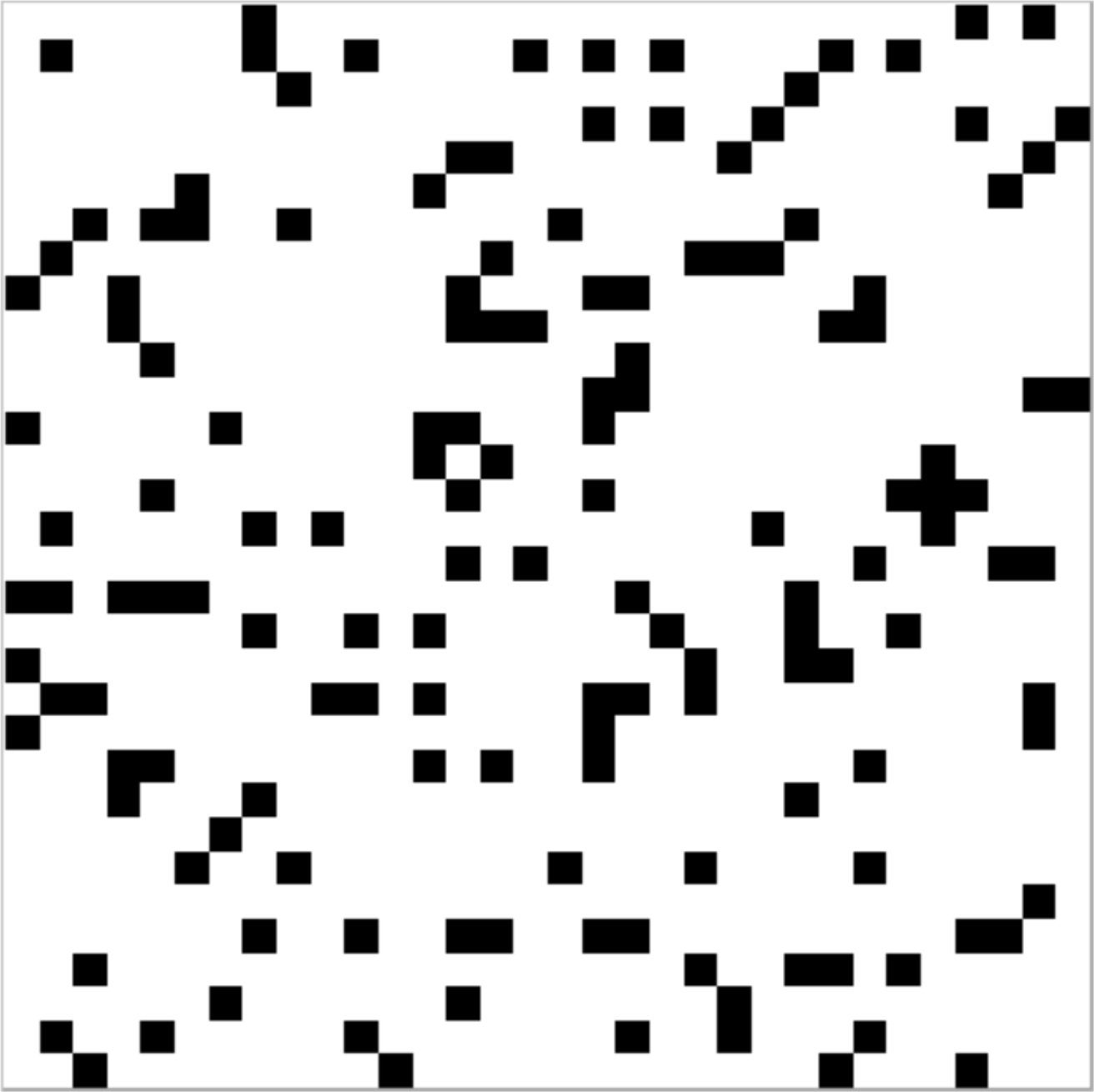
When implementing cellular automata within Turtle, it often makes sense to change the resolution of the canvas image (as well as the virtual canvas dimensions) so that each cell corresponds to a single “pixel” (as well as a single coordinate location). Then the cell’s colour can easily be set using the pixset command, as in the following simple Turtle Pascal program (LifeStart) which creates an initial setup for the Game of Life – an example result is shown in the image.
PROGRAM LifeStart;
CONST width = 32;
      height = 32;
VAR x, y: integer;
BEGIN
  canvas(0, 0, width, height);
  resolution(width, height);
  for x := 0 to width - 1 do
    for y := 0 to height - 1 do
      if random(7) = 0 then
        pixset(x, y, black)
      else
        pixset(x, y, white)
END.
Use of the two constants width and height – both here set to 32 – makes this code very easily adaptable for different sizes of board, just by setting the constants to different values. The canvas command then specifies the relevant coordinate range (i.e. 0 to 31 along both axes) and the resolution command fixes the corresponding image size (i.e. 32×32 pixels). Then the two variables x and y are used to count through all the cells in turn, randomly making roughly one in seven of them black and the rest white (though in fact there would be no need to set the latter, because white is the default colour). And just as the pixels’ colour can be set with the pixset command, so the pixcol function can be used to read that colour, e.g. thiscol := pixcol(x,y). As we shall see, this makes it possible to use the pixel colour itself to record the state of each cell.
4.2 Modelling the Spread of Disease, and Its Prevention
Before tackling the complexities of the Game of Life, it will be helpful to start with a much simpler cellular automaton, and one which – somewhat ironically – is far more closely related to real life! The Disease example program is an implementation of the famous “SIR” (Susceptible, Infected, Recovered) model of the spread of infectious disease, and conveys some very important practical lessons about disease prevention. The program begins by defining various constants:
- Canvas dimensions
widthandheight(both 100 in this case). - Colours to indicate cells that are
susceptible(lightgreen),infected(red), andrecovered(blue). - An integer
startradius(10) that defines the maximum boundary of the initial infection. - Three probabilities, each of which is to be interpreted as a percentage:
infectprob(1%), the probability that a cell withinstartradiuswill be initially infected;immuneprob(2%), the probability that a cell will be immune throughout (e.g. due to prior inoculation); andrecoverprob(15%), the probability that an infected cell will recover in any time period.
As before, the point of defining these constants (rather than using the numbers directly in the code) is to make them very easy to change, so you can experiment with different values. The whole point of this program, indeed, is to see how the behaviour then changes.
Following the constants and a few variables – including numinfected, which keeps count of infected cells – there is a simple procedure infect(x,y), which colours cell (x,y) with the infected colour (i.e. red) and increments numinfected accordingly. Then the main program begins, defining the canvas and resolution (just as we saw above), initialising numinfected to zero, and colouring the cells of the canvas according to the following rules:
- If a cell’s distance from the centre of the canvas is less than or equal to
startradius(10), then with probabilityinfectprob(1%), it will beinfected(red) from the start. - Otherwise, with probability
immuneprob(2%), the cell will berecovered(blue) from the start – this colour is given to cells that are immune, mostly after recovery from the infection. - Otherwise, the cell will be
susceptible(lightgreen).
The canvas is temporarily frozen (using noupdate … update) while this colouring is taking place, so it can be completed much more quickly.
Having finished this initialisation, the spread and eventual decline of the infection are modelled with a loop that continues until numinfected becomes zero. The loop starts by choosing a random value of x between 0 and (width-1) and a random value of y between 0 and (height-1). Then we check the colour of cell (x,y) to see whether it is infected (i.e. red) or not. If it is, then with probability recoverprob (15%), we change it to recovered (i.e. blue), to indicate that it has now recovered and thus become immune from further infection. (To do this with the correct probability, we use the conditional if random(100)<recoverprob to select a random number between 0 and 99 and check whether it is less than recoverprob.) Finally, if the cell is infected and has not recovered, then the following code is executed:
n :=random(4) * 2 + 1;
x := x + n div 3 - 1;
y := y + n mod 3 - 1;
if pixcol(x, y) = susceptible then
  infect(x, y);
The purpose of this code is to select at random one of the four closest neighbours of the infected cell and then, if that cell is susceptible (i.e. lightgreen), to infect it – this is how the infection spreads. The arithmetic here is neat but a bit tricky, going through the following steps and using the operators for integer division (div) and remainder (mod):
random(4) | random(4) * 2 | n | n div 3 | n div 3 - 1 | n mod 3 | n mod 3 - 1 |
|---|---|---|---|---|---|---|
| 0 | 0 | 1 | 0 | -1 | 1 | 0 |
| 1 | 2 | 3 | 1 | 0 | 0 | -1 |
| 2 | 4 | 5 | 1 | 0 | 2 | 1 |
| 3 | 6 | 7 | 2 | 1 | 1 | 0 |
The first, fifth, and last columns show the four possible random numbers (between 0 and 3), and the corresponding values that get added to x and y respectively. Adding (-1,0) corresponds to a move left on the canvas, (0,-1) to a move up, (0,1) to a move down, and (1,0) to a move right. So after these additions, the coordinates (x,y) do indeed identify one of the four neighbouring cells. Now it just remains to test whether that cell is susceptible (lightgreen), and if it is, to infect it (red).
You might have noticed that moving in these ways from a cell on the edge of the grid could take us to a pixel off the canvas. One convenient feature of
pixsetandpixcol– unlike corresponding operations with arrays – is that they do not throw up an error message if this happens, and since it causes no trouble for the operation of our program, we are able to ignore this complication here. But an inquisitive student might want to investigate whether changing the colours could introduce a problem …

One practical virtue of this model of infection – which in its more sophisticated forms is highly influential and widely used – is to demonstrate very clearly the value of inoculation. If the program is run as it stands, the infection is very likely to spread from the centre of the canvas to most of the susceptible cells (the image above shows it spreading aggressively in several directions). But if the value of immuneprob is set higher – for example, changed from 2% to 12% – then you will find that the infection has far less impact, often dying out quickly and usually reaching only a small proportion of the canvas. Thus artificially inoculating even 10% of the population can potentially bring a huge payoff in disease control for the population as a whole. Real diseases, of course, will vary in infectivity and other characteristics, so we cannot assume that this conclusion will apply to them. But this model does allow for variation, and enables us to explore how the critical value of immuneprob at which the disease can be tamed depends on the probability of recovery in each time period: if recovery typically takes a long time (because recoverprob is low), then more widespread prior immunity will be required to keep the disease in check. The crucial point here is that the longer recovery takes for any individual, the more opportunity the disease has to infect that individual’s neighbours, and so the higher the probability that it will indeed be passed on to them.
This particular population structure – which assumes that every individual is statically located within a fixed grid, with precisely four neighbours each – is of course very crude, but more complex versions of the “SIR” model play a vitally important role in the real world, helping epidemiologists (those who study such things) to understand, predict and combat the spread of diseases. In the mathematics of infection, the most important parameter for any disease is its “basic reproduction number” (commonly denoted ) – that is, the number of individuals that could be expected, on average, to be directly infected from one newly-infected individual within a totally susceptible population. In our model (with recoverprob at 15%), this parameter is around 2.35 for an individual surrounded by four “susceptibles”, but of course any individual thus infected will then have only three adjacent susceptibles (since the individual who infected them is no longer susceptible), and their expected direct infectivity drops accordingly, to around 1.76. An interesting experiment would be to see what happens if individuals are allowed to wander (e.g. perhaps by incorporating the sort of “diffusion” modelled in the next chapter), in which case the spread of disease is likely to be significantly greater. In general, if a population is “well mixed”, then an infection is likely to become an epidemic if its numbers systematically grow, i.e. if is greater than 1.
4.3 The Game of Life
The most famous cellular automaton, and one of the most fascinating, is John Conway’s Game of Life. This involves a square grid of cells – potentially extending for ever in all directions – within which each cell can be either alive or dead (so there are just two possible cell states). Since an infinite grid is impractical, most computer implementations involve instead a finite square grid, e.g. 50×50, with the edges “wrapping around” (so the right-hand column is treated as being adjacent to the left-hand column, and the bottom row adjacent to the top row). Within this grid, live cells are usually shown black, and dead cells white – the initial arrangement of these black and white cells may be set randomly (e.g. perhaps as we saw earlier, with a 1 in 7 chance of each cell being alive).
| 1 | 2 | 3 |
| 8 | 4 | |
| 7 | 6 | 5 |
Within any such grid, we consider each cell as having 8 neighbour cells, as shown in the table above. (This differs from the disease model above, in which we treated only cells 2, 4, 6, and 8 as neighbours. These are the two most common options, but many models adopt yet other definitions of “neighbourhood”.) What happens to each cell then depends on whether it is alive or dead, and how many of its neighbours are alive or dead. From one generation to the next:
- A cell that is currently alive will stay alive in the next generation if, and only if, it currently has exactly 2 or 3 live neighbours. Otherwise, it dies.
- A cell that is currently dead will become alive in the next generation if, and only if, it currently has exactly 3 live neighbours. Otherwise, it stays dead.
Though simple, however, these rules can be tricky to implement, because of the need to perform them on all cells simultaneously. If A and B are neighbouring cells and we deal with A first, then if A’s state changes as a result, this risks messing up the calculation for B, whose next state should be determined (in part) by A’s current state, not by A’s next state. The upshot is that we need to be able to retain in memory both the current state of each cell, and the newly-calculated state that will take over in the next generation.
4.4 Colour Codes, Binary Numbers, and Bitwise Operators
Just as with our earlier model of disease, so in the Game of Life there is no need to keep a separate record of whether each cell is alive or dead – the pixels store that information already and can be manipulated individually using pixset and pixcol. And in fact the pixels can store far more information that this, because each pixel holds a three-byte RGB colour code, in which the most significant byte (i.e. the one written first, which has the biggest impact on the overall size of the hexadecimal number) represents the intensity of red, the middle byte the intensity of green, and the least significant byte the intensity of blue (this is exactly the same colour coding method that is used in web pages). Thus for example the colour emerald has colour code #00C957, with # indicating that the number is hexadecimal (base 16), so that the red component is #00 (zero), the green component is #C9 (12×16 + 9 = 201 in decimal), and the blue component is #57 (5×16 + 7 = 87 in decimal). Since the maximum possible value for any component is #FF (15×16 + 15 = 255 in decimal), we can see that emerald is overall mostly green, mixed with some blue.
To get hold of the individual bits and bytes of colour codes (or any other number), we need to understand how they are stored within the computer as binary (base 2). Consider again the code for emerald, divided into hexadecimal digits, each of these corresponding to a 4-bit chunk or nybble:
| Hexadecimal (#) | 0 | 0 | C | 9 | 5 | 7 |
|---|---|---|---|---|---|---|
| Binary | 0000 | 0000 | 1100 | 1001 | 0101 | 0111 |
The four binary digits of each nybble count for 8, 4, 2, and 1 respectively, and we call this their place value (in our familiar decimal system, of course, the place values – starting from the right – are 1, 10, 100 etc.). Thus the binary number “1001” is equivalent to decimal “9” (8+1), “0111” to decimal “7” (4+2+1), “0101” to decimal “5” (4+1), and “1100” to decimal “12” (8+4). The highest possible value for a nybble is thus decimal “15” (“1111” = 8+4+2+1), so a nybble can take any value between 0 and 15, which enables it to be represented by a single hexadecimal digit (just as any value between 0 and 9 can be represented by a single decimal digit). Use of hexadecimal obviously requires that we have 16 different digits available, and that’s why we go beyond “9” to use “A” as the hexadecimal digit for 10, “B” for 11, “C” for 12, “D” for 13, “E” for 14, and “F” for 15. (In the table above, notice that the binary number “1100” – value 8+4 – corresponds to the hexadecimal digit “C”.)
Once we understand binary numbers, we can make use of bitwise operators to manipulate them. Turtle provides four such standard operators, which are called:
not | and | or | xor | (Pascal and Python) |
NOT | AND | OR | EOR | (BASIC) |
The not operator inverts the bits of the integer to which it is applied, taking it to have 32 bits altogether (see the box in §3.3 above), rather than only the 24 bits that are taken into account in colour codes. Thus not(0), for example, will give #FFFFFFFF in hexadecimal, all 1-bits in binary (which in the two’s complement system – also mentioned in the box in §3.3 above – happens to represent the integer -1). The other three operators fix each bit in accordance with the following truth-tables:
These truth-tables fit with the natural “logical” interpretation of the three operators, taking 0 as
falseand 1 astrue(e.g.A and Bcomes out true only if bothAandBare individually true). Hence in Turtle these operators can be used both as “logical” connectives (connecting two statements) and “bitwise” operators (on two numbers).
| A | B | A and B |
|---|---|---|
| 1 | 1 | 1 |
| 1 | 0 | 0 |
| 0 | 1 | 0 |
| 0 | 0 | 0 |
| A | B | A or B |
|---|---|---|
| 1 | 1 | 1 |
| 1 | 0 | 1 |
| 0 | 1 | 1 |
| 0 | 0 | 0 |
| A | B | A xor B |
|---|---|---|
| 1 | 1 | 0 |
| 1 | 0 | 1 |
| 0 | 1 | 1 |
| 0 | 0 | 0 |
So if, for example, we apply these operators between the decimal numbers 21 (binary 00010101) and 9 (binary 00001001), we get:
00010101 (21) 00010101 (21) 00010101 (21)
00001001 (9) 00001001 (9) 00001001 (9)
and: 00000001 (1) or: 00011101 (29) xor: 00011100 (28)
(21 and 9) yields 1, because the only 1-bits in the result are those that were 1-bits in both of the original numbers. (21 or 9) yields 29, because the only 0-bits in the result are those that were 0-bits in both of the original numbers. (21 xor 9) yields 28, because the 1-bits in the result are those that were a 0-bit in one of the original numbers, and a 1-bit in the other.
Suppose now that we are given some six-digit hexadecimal colour code #RRGGBB and we want to get hold of the green component – the middle 8 bits (2 nybbles). We can do this by anding with the hexadecimal number #00FF00, which has all 1-bits in the middle byte and 0-bits elsewhere, and then dividing by #100 (i.e. 256 in decimal). Thus
(emerald and #FF00) evaluates to #C900 (in hexadecimal)
((emerald and #FF00) / #100) evaluates to #C9 (in hexadecimal, 201 in decimal).
If on the other hand we wish to add an element of red (say an intensity of 8/255) to emerald (#00C957), then we can do this using the or operator:
(emerald or #80000) evaluates to #08C957
In this way, the and operator can be used to discover which bits are “set” (i.e. are 1-bits) in the binary representation of a number, and the or operator can be used to ensure that specific bits get set. The xor operator is useful when we want to change a particular bit (from 0 to 1, or 1 to 0).
4.5 Life, Hiding in the Pixels
Let’s now see how we can implement the Game of Life, storing all the intermediate information in the pixels. This incidentally provides a nice illustration of the techniques explained above, which can also be used for steganography, in which secrets are hidden in what look like ordinary pictures (which is a fun topic to be explored in future Turtle materials).
So far, we have two colour codes in our Game of Life pixels, black and white. Spelled out in binary, with all 24 colour bits represented by a digit, black is “000000000000000000000000” and white is “111111111111111111111111”; so it clearly makes life easier if we work in hexadecimal!
black (live cells): #000000 – zero intensity of red, green, and blue
white (dead cells): #FFFFFF – maximum intensity of red, green, and blue
Every bit of black is 0, and every bit of white is 1, but instead of using the entire number to indicate whether each cell is currently alive or dead, we could use just a single bit, for example the least significant bit (the very last, whose place value is 1). And then we could use the next least significant bit (the second last, whose place value is 2) to indicate something quite different, namely, whether the cell is going to change state in the next generation. So now we can add two new colour codes:
blackish (live but dying): #000002 (last byte is 00000010 in binary)
whitish (dead but resurrecting): #FFFFFD (last byte is 11111101 in binary)
Visibly, blackish will be indistinguishable from black, and whitish will be indistinguishable from white. So we can store this information as we go along, without affecting how the canvas looks! Changing a code from black to blackish, or white to whitish – or reversing such a change – is easily done by xoring the code with the number 2, for example (black xor 2) = blackish, and (blackish xor_2) = _black.
When calculating which cells are to die or be resurrected, we need to go through every cell in the grid, applying the rules we saw before:
- A cell that is currently alive will stay alive in the next generation if, and only if, it currently has exactly 2 or 3 live neighbours. Otherwise, it dies.
- A cell that is currently dead will become alive in the next generation if, and only if, it currently has exactly 3 live neighbours. Otherwise, it stays dead.
Recall also that every cell has 8 neighbouring cells, even those on the edges of the grid, because the grid “wraps around” from left to right, and from top to bottom. Perhaps surprisingly, this wrapping around is very straightforward, because we can take advantage of the mod operator (written “MOD” in BASIC) which yields remainders (e.g. 14 mod 4 = 2, because 4 goes into 14 three times, with a remainder of 2). If we’re concerned with cell (x,y) and use variable dn to count “dead neighbours”, then the code (in Pascal) might go like this:
var dn, i, j: integer;
…
dn := 0;
for i := -1 to 1 do
for j := -1 to 1 do
dn := dn + pixcol((x + i + width) mod width,
(y + j + height) mod height) and 1;
Suppose for example, that x is 31 and y is 0 on a 32×32 grid, so the pixel (x,y) is at the top-right corner. Then as i and j both count from -1 to 1, the expression “(x+i, y+j)” passes through 9 combinations of coordinates (including (31, 0) itself when both i and j are zero):
(30, -1) (31, -1) (32, -1) j = -1; y+j = -1
(30, 0) (31, 0) (32, 0) j = 0; y+j = 0
(31, 1) (31, 1) (32, 1) j = 1; y+j = 1
i = -1; x+i = 30 i = 0; x+i = 31 i = 1; x+i = 32
The shaded combinations are not legitimate gridpoints, because the coordinates in each direction run only from 0 to 31, so both -1 and 32 are “illegal” values. But suppose now that we do the following to the coordinates within each pair – add 32, then take the remainder on division by 32. The effect on the numbers shown above is as follows (using mod as the remainder function):
| n | -1 | 0 | 1 | 30 | 31 | 32 | |
|---|---|---|---|---|---|---|---|
| n + 32 | 31 | 32 | 33 | 62 | 63 | 64 | |
| (n + 32) mod 32 | 31 | 0 | 1 | 30 | 31 | 0 |
Notice how -1 has “wrapped around” to 31, and 32 to 0, while the four legitimate values are unaffected. This changes our 9 combinations of coordinates to exactly what we want them to be:
(30, 31) (31, 31) (0, 31)
(30, 0) (31, 0) (0, 0)
(31, 1) (31, 1) (0, 1)
Thus our command:
dn := dn + pixcol((x + i + width) mod width,
(y + j + height) mod height) and 1;
does check the correct neighbourhood of pixels around (x,y), both at the edges and in the middle of the grid (and it’s written in such a way that width and height could take values other than 32).
Now let’s look at what’s happening to dn. This is first set to 0, and then gets repeatedly incremented by (pixel and 1), where pixel is in turn the colour code of the 9 cells in the neighbourhood of (x,y) – i.e. cell (x,y) itself and its 8 neighbours. “(pixel and 1)” applies the and operator between pixel and #000001, thus yielding the value of the least significant bit, which is what we are using to record whether the cell is alive or dead (and note that we could equally well have used “(pixel mod 2)” here, because the last bit is 1 if and only if pixel is odd). If the cell is alive, and pixel is black or blackish, then pixel is even, so (pixel and 1) will be 0. If dead, and pixel is white or whitish, then pixel is odd, so (pixel and 1) will be 1. Hence the command above does indeed succeed in counting the number of dead cells in the neighbourhood (and its doing so will be unaffected if some of the cells change colour from black to blackish, or from white to whitish). Having counted the number of dead cells, it’s easy to modify the Game of Life rules accordingly:
- A cell that is currently alive will stay alive in the next generation if, and only if, there are currently 5 or 6 dead cells (i.e. 4 or 3 live cells) in the neighbourhood. Otherwise, it dies.
- A cell that is currently dead will become alive in the next generation if, and only if, there are currently 6 dead cells (i.e. 3 live cells) in the neighbourhood. Otherwise, it stays dead.
Applying these rules to cell (x,y) can now be done as follows, bearing in mind that (black xor 2) is blackish, and (white xor 2) is whitish. We want to make these colour changes (signifying an impending change of state) if either cell (x,y) is alive but the neighbourhood has neither 5 nor 6 dead cells, or if cell (x,y) is dead and the neighbourhood has exactly 6 dead cells:
if ((pixcol(x,y) and 1=0) and ((deadns<5) or (deadns>6)))
or ((pixcol(x,y) and 1=1) and (deadns=6)) then pixset(x,y,pixcol(x,y) xor 2);
If we go through all the cells in the grid, performing these steps, then by the time we have finished, we will still have a grid that looks exactly the same (since blackish is indistinguishable from black, and whitish from white), but in which every cell that is due to change from live to dead, or vice-versa, will actually have subtly changed colour. And we will have done all this without allowing the calculations on each cell to affect those on its neighbours. All that remains, to finish this “generation” of the Game of Life, is to go through the entire grid updating blackish (i.e. dying) to white (i.e. dead), and whitish (i.e. resurrecting) to black (i.e. alive). This can be done routinely:
if pixcol(x,y)=#2 then
pixset(x,y,white)
else
if pixcol(x,y)=#FFFFFD then
pixset(x,y,black)
or more cleverly, with bitwise operations:
if (pixcol(x,y) and 3) mod 3<>0 then
pixset(x,y,pixcol(x,y) xor #FFFFFD)
This uses the fact that blackish differs from white, just as whitish differs from black, in every bit except for the second last. So xoring with #FFFFFD – which has every bit set except for the second last – accomplishes exactly the changes we want. To test for the cells which need to be updated, we take the bottom two bits of the pixel colour (by anding with 3), and then find the remainder when this number is divided by 3. If the two bits are the same, then they make either 0 or 3 (00 or 11 in binary), hence zero remainder. If the two bits are different, we get a remainder of either 1 or 2, so we know that the current colour cannot be black or white; hence updating is needed. Having completed all these updates, we will be ready to start again on the next generation, and by putting the whole thing within a continuous loop (e.g. “while ?key<>\escape do”, which will keep going until the ESCAPE key is pressed), we finish our implementation of the Game of Life.
This full implementation of the Game of Life is available – in BASIC, Pascal, and Python – within the Help menu of each language.
4.6 Investigating One-Dimensional Cellular Automata
The simplest cellular automata have two possible states per cell (like the Game of Life) but are only one-dimensional, meaning that all the activity takes place along a single line. Though simple, however, this brings a new element of interest for us, because it enables us to picture what happens through the generations, by showing them on successive lines of the canvas. As usual, we’ll fix the states of the first generation of cells (along the top line of the canvas) randomly.
Suppose we consider the states as 0 and 1 – showing as white and black respectively (though we’ll use the visually indistinguishable #FFFFFE for white and #000001 for black, so that the bottom bit of each colour code yields 0 and 1 respectively). If we take the neighbourhood of each cell to consist of itself and the two adjacent cells, then there are eight possibilities for each neighbourhood:
111 110 101 100 011 010 001 000
Depending on the nature of our automaton’s transition rule – which is assumed to be deterministic (i.e. not chancy) – each of these possibilities will lead to one of two specific outcomes in the next generation, making the cell in question (i.e. the middle one of the three) either 0 or 1. For example, our rule might specify the following transitions for the eight possible neighbourhood situations:
111 110 101 100 011 010 001 000
(R) 0 1 1 0 1 1 1 0
Suppose we apply this rule to a first line that has randomly turned out like this:
| 1 | 1 | 1 | 0 | 1 | 0 | 0 | 0 | 1 | 1 | 0 | | — | — | — | — | — | — | — | — | — | — | — |
The rule depends on 3-cell neighbourhoods, but the two end cells don’t have such a neighbourhood (because they have only one neighbour); hence we imagine the line “wrapping around” so that the “0” at the right-hand end is considered as adjacent (on the left) to the “1” at the left-hand end:
| 0 | 1 | 1 | 1 | 0 | 1 | 0 | 0 | 0 | 1 | 1 | 0 | 1 | | — | — | — | — | — | — | — | — | — | — | — | — | — |
Then the result for each of the cells, derived by examining its 3-cell neighbourhood and consulting the relevant part of the rule, will be:
| 1 | 0 | 1 | 1 | 1 | 0 | 0 | 1 | 1 | 1 | 1 | | — | — | — | — | — | — | — | — | — | — | — |
Thus in the first cell, we see “011” leading to “1”; in the second, we see “111” leading to “0”; in the third, we see “110” leading to “1”; in the fourth, we see ““101” leading to “1”, and so on.
Of course this is only one possible transition rule, and since there are two possible transitions for each of eight possible neighbourhood situations, it follows that there are – i.e. 256 – possible rules altogether. Specifying these rules is very simple, because each transition is to either “0” or “1”, so each such choice can be treated as a binary digit, giving us rules numbered from “0000000” (zero) to “11111111” (255 in decimal). And we can see from (R) above that by this method, the illustrated rule is number “01101110” in binary, or 110 in decimal.
The example program “Automata” (pictured here having processed rule 110) counts through an interesting subset of these 256 rules, and it can easily be modified to count through all of them. The setup procedure takes this numeric rulecode as a parameter, and identifies each of its binary digits in turn (by finding the remainder on division by 2, then executing rounded-down integer division by 2 and continuing). Each of these digits is stored in the nextstate array, so nextstate[5], for example, will then specify the required transition for the neighbourhood “101” (which is 5 in binary).
The main program begins by defining the canvas and resolution dimensions as width×height in the usual way, and putting appropriate colour codes (#FFFFFE and #1 respectively) into the array elements cellcol[0] and cellcol[1], so that the binary digit resulting from any transition can easily be translated into a pixel colour. Then comes a for loop which sets the variable n counting from 4 to 45, while in turn rule is made equal to (4n+2), so that rule counts from 18 up to 182 in steps of 4 (these numbers just happen to give an interesting subset of rules). Each time round the loop, the canvas is cleared to white, and the cells in the top line – generation 0 – are filled randomly with either cellcol[0] or cellcol[1]. The rest is then filled in by repeated calls of the nextgen procedure, implementing the generations from 1 to the bottom of the canvas (so the number of the final generation is height-1).
Procedure nextgen takes the generation number, g, as a parameter, and counts through the pixels on canvas row g-1 (i.e. the parent row), working out which transitions should be applied to create the pixels on row g. Although the parent pixels are indexed horizontally from 0 to width-1, this count is extended at each end, going from -1 to width, to capture all the 3-cell neighbourhoods using the remainder operator mod in something like the now familiar way:
for x:=-1 to width do
begin
xmod:=(x+width) mod width;
thispix:=pixcol(xmod,g-1) and 1;
n3:=n2*2+thispix;
n2:=n1*2+thispix;
n1:=thispix;
if x>0 then
pixset(x-1,g,cellcol[nextstate[n3]])
end
At the extremes, when x is -1, xmod will be (width-1), and when x is width, xmod will be 0; in all other cases, x and xmod are equal. This means that as x counts from -1 to width, xmod will count from (width-1) to 0, wrapping round from the right-hand edge of the canvas to the left, and thus including the full neighbourhood of both extreme cells. As this count proceeds, thispix becomes either 0 or 1, depending on the pixel value of the relevant cell (with “and 1” ensuring that we take only the last binary digit – as we saw with the Game of Life, “mod 2” would have exactly the same effect). Then, treating the next three lines in reverse, n1 is made equal to thispix, n2 is made equal to thispix plus twice the previous value of n1, and n3 is made equal to thispix plus twice the previous value of n2. So after we have gone round this loop three times – and using p[n] here to signify the value (i.e. 0 or 1) of the nth pixel on row (g-1) – these variables will be set as follows:
x: 1 n1: p[1] n2: p[0]×2 + p[1] n3: p[width-1]×4 + p[0]×2 + p[1]
Thus n3 will now have a value which, in binary, reflects the neighbourhood of cell 0 in generation (g_1). And so to apply the necessary transition rule, we make the next-generation cell at (0, _g) equal to nextstate[n3], and set the corresponding pixel colour to cellcolour[nextstate[n3]]. Meanwhile, n2 and n1 are primed to go round the loop again, so as to recalculate n3 to give the neighbourhood of cell 1 next time (when x=2), and so on all the way to cell (width-1), whose neighbourhood transition will be applied when x finally reaches width (at which point xmod will have wrapped round to 0).
Following the calculation of the remaining generations, the program ends by displaying the rule number, at the bottom left of the canvas:
setxy(0,height-15);
box(25+length(str(rule))*7,14,cream,false);
print('Rule '+str(rule),4,8);
This first moves the turtle to location (0,85), assuming the height is 100. Then it draws a cream-coloured “box” (without a border), whose height is 14 pixels and whose width is:
25+length(str(rule))*7.
Depending on whether the rule number has 1, 2 or 3 digits, this gives a box width of 32, 39, or 46 respectively. Then we print “Rule 110” (or whatever) in Turtle font number 4 (Comic Sans) and size 8. As can be seen in the image of rule 18 below, this gives as neat a finish with a two-digit number as we saw before with three.
4.7 Cellular Automata, Patterns in Nature, and Alan Turing
If we compare the pattern produced by rule 18 with the pattern on the shell of a Conus textile sea snail (both are pictured here), one cannot but be struck by their amazing similarity. This seems unlikely to be coincidence, especially when we consider that the snail’s shell has been built up through growth along the line of its edge, so that its pattern is the result of a sequence of lines generated through time, just like our cellular automaton patterns.
 In 1952, Alan Turing published a paper on “The Chemical Basis of Morphogenesis”, in which he hypothesised a “reaction/diffusion” process for the creation of biological patterns such as on the coats of zebras and leopards. In recent years, this theory has inspired cellular automaton models that work in a functionally similar way, and the use of such models to investigate the formation of patterns in nature has become a significant area of fascinating research.