3. Computing in Physics: Cannons and Rockets

3.1 Applying Gravity

We can now try producing some physical simulations to illustrate basic principles of mechanics, focusing on the motion of projectiles. If we assume that these are sufficiently heavy and streamlined to ignore the effects of air resistance, then the most important principles are the following, which relate to Newton’s first and second laws of motion:

(H) Gravity does not directly affect horizontal motion, which will continue at uniform velocity unless acted upon by some other force.

(V) Gravity imposes a constant vertical acceleration towards the ground.

We have already seen how moving objects can be easily modelled in terms of horizontal and vertical movement; here we do the same again, with xvel being constant (by principle H) and yvel changing with gravity (by principle V).

To model motion under gravity precisely, we would need to calculate its effect continuously rather than discretely, and this would involve using the mathematics of calculus (differentiation and integration). Our aim here, however, is not to be precise, but rather to get an intuitive understanding of the principles, and sufficient realism to illustrate the physics (and perhaps to use in our own video games). So as before with the bouncing ball, we imagine the motion taking place in successive “cycles”, where each cycle takes enough time for some significant distance (e.g. several units of the canvas) to be covered. This means that as a projectile falls to the ground – getting faster and faster and covering more vertical units each cycle – it is unlikely to reach exactly ground level at the end of a cycle: it is more likely to overshoot. This will need correcting (by treating the ground level as a minimum), unless we are happy for our cannonball (or whatever) to dig a hole.

Bearing all this in mind, and using the turtle itself to execute the movement, here is a simple procedure for modelling the flight of a small red ball under gravity, expressed in Turtle Pascal (the Turtle BASIC and Turtle Python versions are very similar).

Procedure throwball(xvel, yvel, gravity, floor: integer);
Begin
  repeat
    noupdate;
    colour(white);
    blot(25);
    movexy(xvel, yvel);
    yvel := yvel + gravity;
    if turty > floor then
      turty := floor;
    colour(red);
    blot(25);
    update;
    pause(10)
  until turty = floor
End;

The procedure takes four parameters, representing the initial x-velocity and y-velocity of the ball, the gravitational acceleration (per cycle), and the floor of the motion (so that if the turtle y-coordinate turty gets below floor level, it gets made equal to the floor level instead). Note that gravity acts downwards, and is therefore added to the y-velocity (given that the y-axis points downwards in computer graphics, unlike standard school maths).

To see this gravitational procedure in action, look at the Movement under gravity example that can be found in the Help menu of each language.

3.2 Plotting Cannonball Flight

The AimCannon example program uses exactly the same technique to model the flight of a cannonball – the only significant difference in its “fire” procedure is that this is designed to avoid leaving a visible trail as the ball passes along the gun barrel and its surround (by testing the colour of the relevant pixel before drawing: the black ball is drawn only on a white background or when it hits the ground, and erasure takes place only when the black ball has indeed been drawn). The program also has an “aim” procedure which works by detecting any mouse-click on the cream-coloured part of the gun surround, and then turning the gun accordingly:

repeat
until (?lmouse > 0);
if pixcol(?mousex, ?mousey) = cream then
  turnxy(?mousex - 250, ?mousey - 9750);

The (empty) repeat loop keeps checking for a click of the left mouse (when the query code ?lmouse will return a value greater than 0), after which the pixel where the mouse click takes place is tested, and if it is coloured cream, the gun – whose pivot is at position (250,9750) – is turned towards it (by pointing the turtle parallel to the relevant vector and drawing a line of length gunlength). This repeat loop is placed inside another, which exits when the red gun ignition button is clicked.

The AutoCannon program is based on the same principles, but automatically moves the cannon through angles of elevation from 0 to 90 degrees, shooting as it goes and plotting both the distance (in pixels) and the time of flight (in cycles). The result is shown here:

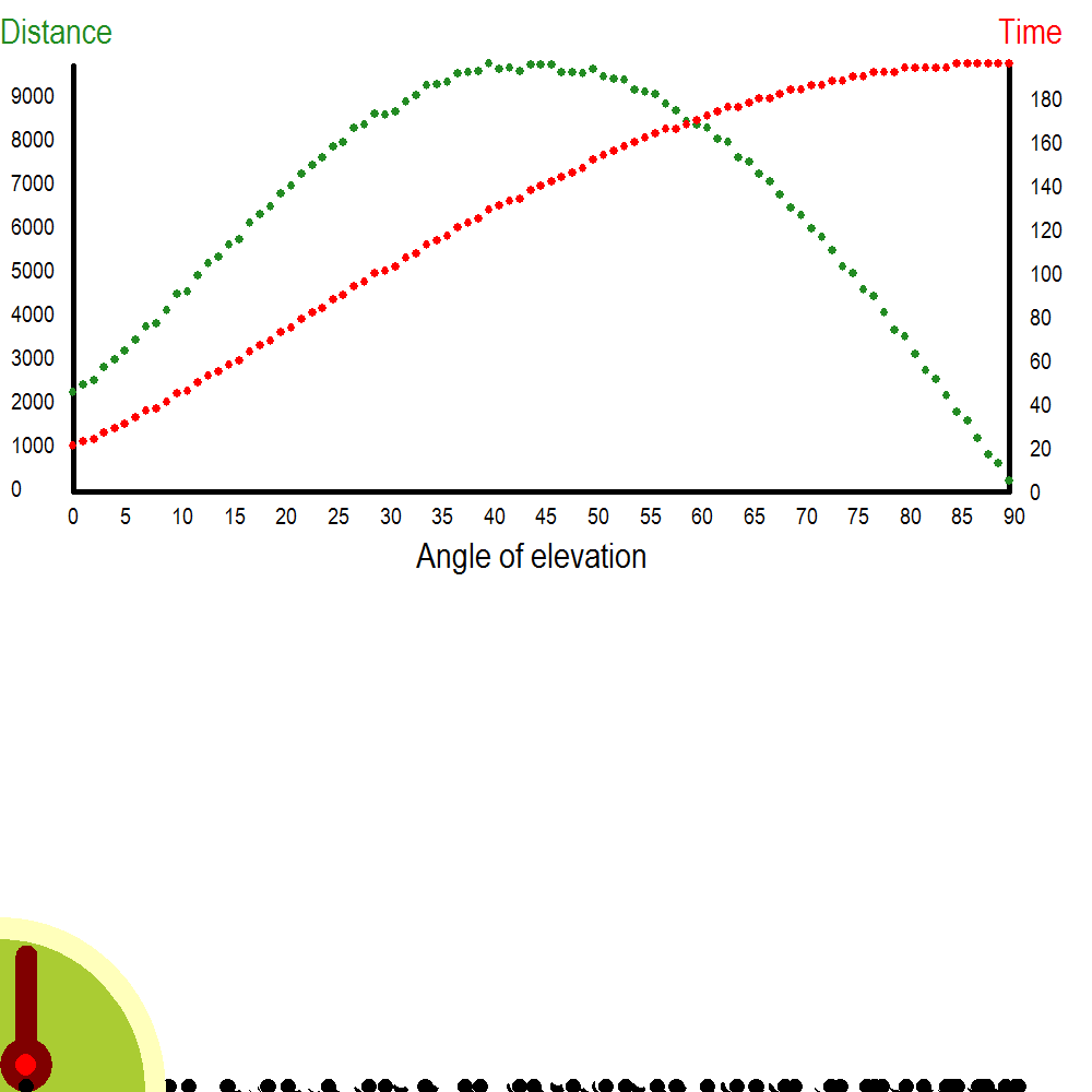
Notice that the ground is littered with old cannonballs, many damaged as more recent shots passed over them (being erased as they went). The graphs at the top of the image illustrate that even though this technique of modelling projectile flight is rather crude and imprecise, it yields behaviour fitting pretty well with the smoothly curved functions of theoretical analysis, with a maximum distance at around 45° of elevation, and time of flight rising throughout (since a greater component of velocity upward takes the ball higher).

3.3 Shooting for Orbit

The cannon simulation programs do not pretend to model reality at all closely – the firing distance is measured in pixels and the time of flight in cycles. The Launch program is very different in this respect, performing calculations based on real scientifically-established values. As such, it also illustrates how the Turtle System, though confined to integers for its internal workings, can handle “floating point” numbers. Be warned, however, that the following material is quite technical!

The scenario is this: a rocket on the surface of the Earth is pointing upwards with a slight slant to the right (initdirection, expressed in seconds of arc, where 3600 seconds make a degree, and hence there are 1296000 seconds in a circle). The rocket applies a thrust of initthrust, expressed in millinewtons-per-kilogram (where one millinewton-per-kilogram is the force required to accelerate the rocket by one millimetre per second per second). But this thrust lasts only for thrusttime seconds, after which the rocket is in “freefall”, and the aim is to achieve orbit around the Earth. As the rocket rises, the thrust of the engine combines with gravity to give it a particular velocity, which can be analysed as usual into vertical and horizontal components. Leaning only slightly to begin with, the rocket gradually “falls” to the right, so that at each moment its direction (and hence the direction of its engine’s thrust) is determined by the ratio of its vertical and horizontal velocities. To achieve orbit, the rocket must lean sufficiently to acquire plenty of speed around the Earth (so that it “falls” around the Earth rather than onto it). But if it leans too much, then gravity will pull it down towards the Earth too quickly, and it will crash. Likewise, if its initial thrust is too great, or maintained for too long a duration, then the rocket will head out into empty space; but if it is too little, or for too short a duration, then it will fail to achieve orbit, and again will crash. Getting the right combination of angle, thrust, and duration is surprisingly tricky, and it is a challenge to find the combination that yields the best orbit, staying as high as possible above the Earth. The program contains a report procedure to write flight statistics to the output window, called whenever the height of the orbit is either constant or changing direction (i.e. when it is at its lowest or highest). When editing the program, you might find it helpful to call this procedure more often to keep track.

The mathematical heart of the program is within the main loop, with each cycle representing one second of time:

dist := hypot(x, y, 1);
gravity := divmult(earthGM, divmult(dist, 1000000, dist), 1000);
xgravity := -divmult(gravity, dist, x);
ygravity := -divmult(gravity, dist, y);
xthrust := sin(d, 1, thrust);
ythrust := -cos(d, 1, thrust);
xvel := xvel + xgravity + xthrust;
yvel := yvel + ygravity + ythrust;
x := x + xvel / 1000;
y := y + yvel / 1000;
d := arctan(xvel, -yvel, 1);

The distances x and y are measured in metres from the centre of the Earth (though the scale of the canvas image is one kilometre per unit, with the rocket enlarged for visibility). Velocities (and accelerations) are measured more accurately, in millimetres per second (per second), because these have a crucial impact on the rocket’s direction, and this effect multiplies as it continues on its way. As noted above, angles are measured in seconds of arc, with an angles(1296000) command at the beginning of the main program ensuring that this setting will be taken into account in both canvas graphics and trigonometrical functions. The Earth is treated as a perfect globe, radius 6371 kilometres, with gravity acting (in effect) from its centre. But calculating the gravitational force with relative precision requires us to use special built-in functions designed to avoid the “overflow” and large rounding errors that we would get with ordinary arithmetic.

An important point in computer science is that fractional numbers are not stored with perfect precision, but in effect represented by combinations of integers. Many systems provide “floating point” representations to disguise this and simplify their use, whereas Turtle provides routines to handle them explicitly as fractions. Another important point is that the storage of integers themselves is limited. Turtle uses the standard method of providing 4 bytes (32 bits) per integer, giving a range between -2³¹ and 2³¹-1 inclusive. (Turtle also uses the standard “two’s complement” representation, whereby the most significant bit of the 32-bit binary number is used to indicate -2³² rather than +2³², thus allowing negative integers.) The upper limit 2³¹-1 (i.e. 2147483647) is called maxint.

The command dist := hypot(x, y, 1) makes dist equal to the (rounded) distance between (0, 0) and (x, y), calculated by Pythagoras’s Theorem as the hypotenuse of a right-angled triangle. Then gravity := divmult(earthGM, divmult(dist, 1000000, dist), 1000) uses the special divmult function twice, to calculate the gravitational attraction of the Earth on the rocket without causing arithmetical overload. The expression divmult(dist, 1000000, dist) yields the rounded value of (dist / 1000000) × dist, thus effectively squaring dist without too much loss of precision and without causing overload. (Note that the radius of the Earth in metres, squared, is far bigger than maxint, the largest integer that Turtle can handle.) Then the other application of divmult divides this value into earthGM, the Earth’s gravitational parameter (398600.442km³s^-2), with multiplication by 1000 at the end enabling the result to be stored to three decimal places (so the units here are again millinewtons per kilogram (or millimetres per second squared – in these units, the familiar value of 9.8 ms^-2 for the acceleration due to gravity at the Earth’s surface is 9800).

Having found a value for gravity, representing the acceleration on the rocket due to the Earth’s pull, this is divided into components in the x and y directions; for example, the proportion in the x direction is x / dist (remembering that dist is the hypotenuse of the x and y triangle), but made negative because it pulls back towards the centre of the Earth at (0, 0). Next, we calculate the x and y components of the rocket’s thrust (determined by the time t and the rocket’s current direction d), with the function sin(d, 1, thrust), for example, giving the rounded value of sin(d) × thrust. Note again that thrust is made equal to initthrust initially, but becomes zero after thrusttime seconds – both of these values are set as constants at the beginning of the program, and can be adjusted as desired. The rocket’s acceleration in the x and y directions is determined straightforwardly by the sum of the corresponding gravity and thrust components (applying Newton’s second law of motion), so its velocity is then adjusted accordingly (e.g. xvel := xvel + xgravity + xthrust). This new velocity is applied to the rocket’s position (e.g. x := x + xvel / 1000, converting from millimetres to metres) and the angle of flight is adjusted to reflect the relationship between its x and y components (using d := arctan(xvel, -yvel, 1)). (Note here that Turtle’s arctan function takes account of the sign of its first two parameters, not just their ratio, so the resulting angle can point in any direction around the circle and is not confined to the “principal values” of the mathematical arctan function.) Having done all this, we are ready to go round the loop cycle again, drawing the rocket as we go.

3.4 Ideas for Independent Exploration: Shooting Games and Rocket Science

3.4.1 Shooting Games

There are several popular video games that involve shooting missiles from one side of the screen to the other, with the aim of hitting your opponent’s pieces or knocking down walls etc. To implement this sort of game, you can use the keyboard to provide control to the players, with keys at the left-hand end of the keyboard being used by one player, and keys at the right-hand end of the keyboard being used by the other. The built-in Snake example program shows how to put key-press identification commands within a game loop, and also illustrates use of pixel colours to identify collisions. See §2.4.2 above for an explanation of key-press functions, and note that a summary of the facilities for keyboard control is available in the “User Input” panel of the software’s Help1 display (the “Help1” tab is standardly at the bottom of the software window, slightly on the right).

One complication that you might encounter concerns the “overshoot” issue that we dealt with earlier by having a floor parameter to the relevant routine (so that if the projectile went “through the ground”, it could be replaced at ground level). If your overshooting is partly horizontal – for example, your missile is found to have hit your opponent’s wall only after it has gone right through the back of it – then you might want to retrace its path to discover the point of impact and treat it as stopping there. For one way in which this can be done, see the Brownian motion example in the next chapter (and in particular section §5.3, discussing how to handle collisions).

3.4.2 Rocket Complications

Our rocket simulation crudely assumes that the rocket engine delivers a constant acceleration for a fixed time, and then shuts off. In practice, rocket engineers need to take into account that the weight of the rocket reduces significantly as the fuel is burnt – and indeed the fuel necessary to get the rocket into space constitutes a huge proportion of its initial weight. This factor could be added to the model described earlier, and would allow some interesting further explorations. Trying to make the figures realistic will give a great opportunity to explore the relevant issues, such as how much energy can be obtained per kilogram by different types of propellant. Relevant information is easily obtained from the web, for example from the excellent article The Tyranny of the Rocket Equation written by Space Shuttle astronaut Don Pettit (on the NASA website).

Another complication would take into account the rotation of the Earth and the location and direction of the launch. When the rocket takes off, it will already be moving horizontally with the Earth’s rotational speed at that point, and this will be greatest at the equator (which is why most launch sites are located in the tropics). To take full advantage of the Earth’s spin, the rocket must take off in an easterly direction (so if the Sun is rising, the rocket will move towards the Sun with both its own speed relative to the Earth, and the Earth’s rotational speed which is taking the launch site towards the Sun). It would be interesting to compare launching eastward with launching westward by adapting the simulation accordingly.

And if you do all this, you can legitimately claim to have been doing “rocket science”!